Tara Sperber
3 of my favourite graphs
Graph 1
A graph of the American Indian population in the midwest USA.
ggplot(midwest, aes(x = poptotal, y = popamerindian)) + geom_point(colour = "red") + geom_smooth(colour = "yellow") ## `geom_smooth()` using method = 'loess' and formula 'y ~ x'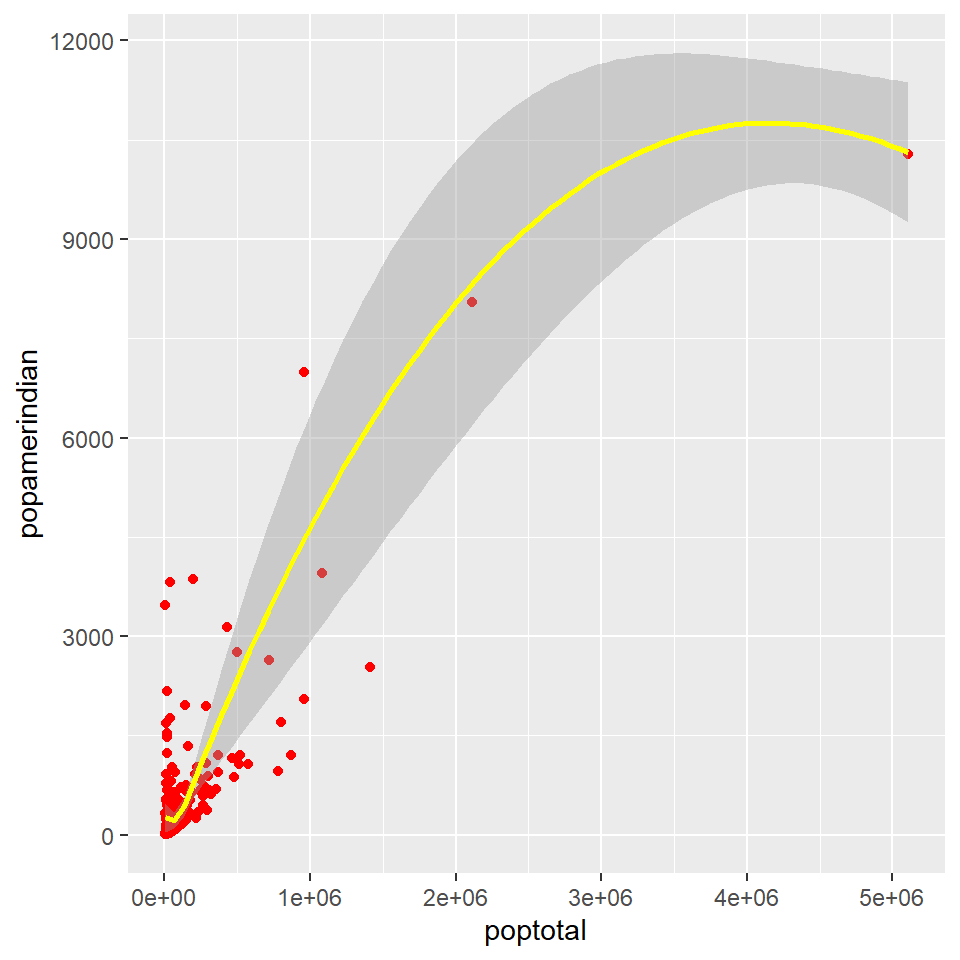
- Graph 2
bbox_l <- bbox <- osmplotr::get_bbox(c(77.56,12.93,77.63,12.96))
bbox_l
## min max
## x 77.56 77.63
## y 12.93 12.96dat_B <- extract_osm_objects(key = "building", bbox = bbox_l) ## Issuing query to Overpass API ...## Rate limit: 2## Query complete!## converting OSM data to sf formatdat_H <- extract_osm_objects(key = 'highway', bbox = bbox_l)## Issuing query to Overpass API ...## Rate limit: 2## Query complete!## converting OSM data to sf formatdat_P <- extract_osm_objects(key = 'park', bbox = bbox_l)## Issuing query to Overpass API ...## Rate limit: 2## Query complete!## converting OSM data to sf formatdat_G <- extract_osm_objects(key = 'landuse', value = 'grass', bbox = bbox_l)## Issuing query to Overpass API ...## Rate limit: 2## Request failed [429]. Retrying in 1.5 seconds...## Query complete!## converting OSM data to sf formatdat_T <- extract_osm_objects(key = 'natural', value = 'tree', bbox = bbox_l)## Issuing query to Overpass API ...## Rate limit: 2## Query complete!## converting OSM data to sf formatBangalore map
This map visualises the highways, parks and trees around Bangalore, my hometown. The gray are the highways, orange the parks and purple are the trees.
tm_shape(dat_B) + tm_polygons(col = "gray40") +
tm_shape(dat_G) + tm_fill(size = 4, col = "orange") +
tm_shape(dat_H) + tm_dots(col = "purple") +
tm_shape(dat_T) + tm_dots(col = "green") +

tm_layout(title = "Bangalore", title.size = 6, frame = TRUE, frame.lwd = 5, bg.color = "lightyellow")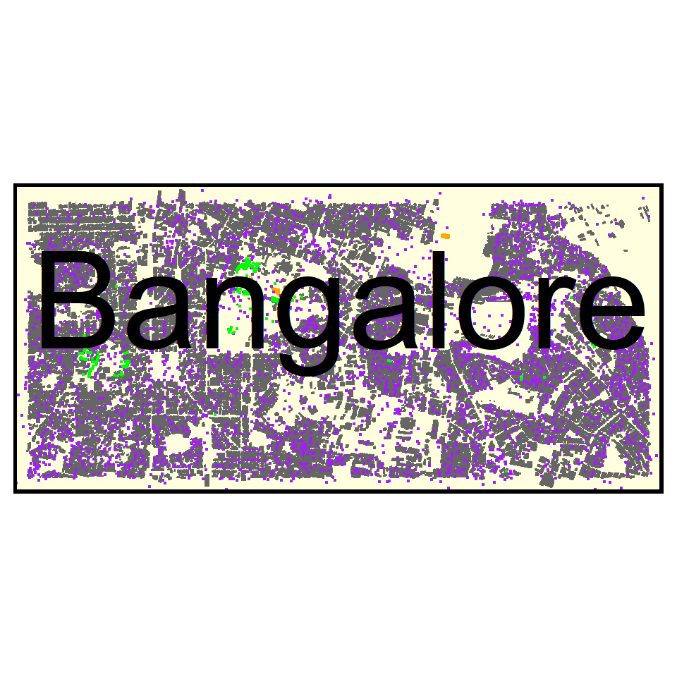
Network Graph
bojack_nodes <- read_csv("./Data/bojack-nodes.csv",trim_ws = TRUE) %>%
  select(1:4) %>%
  drop_na()
## Rows: 15 Columns: 4## -- Column specification --------------------------------------------------------
## Delimiter: ","
## chr (3): Name, Sex, Animal
## dbl (1): Season##
## i Use `spec()` to retrieve the full column specification for this data.
## i Specify the column types or set `show_col_types = FALSE` to quiet this message.bojack_edges <- read_csv("./Data/bojack-edges.csv",trim_ws = TRUE)%>%
select(1:4) %>%
drop_na()## Rows: 20 Columns: 4## -- Column specification --------------------------------------------------------
## Delimiter: ","
## chr (3): from, to, Type
## dbl (1): weight##
## i Use `spec()` to retrieve the full column specification for this data.
## i Specify the column types or set `show_col_types = FALSE` to quiet this message.bojack_nodes## # A tibble: 15 x 4
## Name Sex Animal Season
## <chr> <chr> <chr> <dbl>
## 1 Bojack Horseman male Horse 1
## 2 Princess Carolyn female Cat 1
## 3 Diane Nguyen female Human 1
## 4 Todd Chavez male Human 1
## 5 Mr. Peanutbutter male Dog 1
## 6 Vincent Adultman male Human 1
## 7 Secretariat male Horse 1
## 8 Dick Cavett male Human 1
## 9 Random character female Human 1
## 10 Random character #2 female Human 1
## 11 Sebastian St. Clair male Snow Leopard 1
## 12 Random character #3 male Horse 1
## 13 Lenny Turtletaub male Turtle 1
## 14 Kelsey Jannings female Human 1
## 15 Photographers male Human 1bojack_edges## # A tibble: 20 x 4
## from to weight Type
## <chr> <chr> <dbl> <chr>
## 1 Dick Cavett Secretariat 1 Professional
## 2 Mr. Peanutbutter Bojack Horseman 3 Friends
## 3 Bojack Horseman Todd Chavez 3 Friends
## 4 Princess Carolyn Bojack Horseman 3 Friends
## 5 Vincent Adultman Bojack Horseman 1 Friends
## 6 Vincent Adultman Princess Carolyn 4 Partners
## 7 Mr. Peanutbutter Vincent Adultman 1 Friends
## 8 Princess Carolyn Mr. Peanutbutter 1 Friends
## 9 Bojack Horseman Random character 1 Acquaintance
## 10 Bojack Horseman Random character #2 1 Acquaintance
## 11 Bojack Horseman Random character #3 1 Acquaintance
## 12 Diane Nguyen Photographers 1 Professional
## 13 Diane Nguyen Sebastian St. Clair 2 Professional
## 14 Mr. Peanutbutter Todd Chavez 4 Friends
## 15 Diane Nguyen Mr. Peanutbutter 1 Partners
## 16 Bojack Horseman Lenny Turtletaub 2 Professional
## 17 Bojack Horseman Kelsey Jannings 2 Professional
## 18 Kelsey Jannings Lenny Turtletaub 1 Professional
## 19 Princess Carolyn Diane Nguyen 1 Friends
## 20 Bojack Horseman Diane Nguyen 1 FriendsGraph 3
This graph shows the connections/interactions between characters appearing in Season 1, Episode 12 of Bojack Horseman.
bojack <- tbl_graph(nodes = bojack_nodes,
                    edges = bojack_edges,
                    directed = FALSE)

ggraph(graph = bojack,  layout = "kk") +
geom_edge_link(width = 2, color = "black") +
geom_node_point(shape = 21, size = 8, fill = "pink", color = "red", stroke = 2) 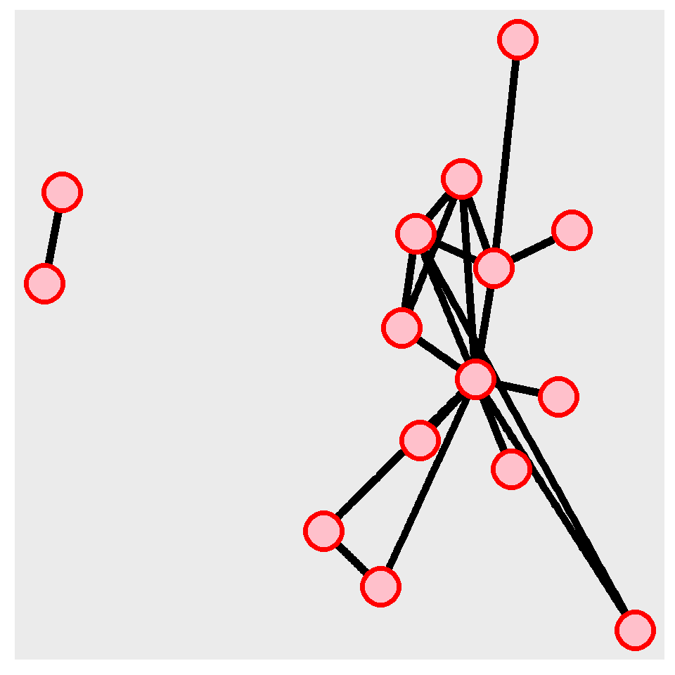
Reflection
Learning this particular language of code was a different experience for me. I’ve had several encounters with code and they were always very stressful. This course was also stressful but one thing different is that I enjoyed learning and working with it.